Tutorial
Here is how to use our package:
For detailed reference of each function please have a look into our Documentation.
For examples check our topoly_tutorial project on GitHub.
Whatever you want to do, start by importing topoly functions:
>>from topoly import *
Accepted structures
Examples: topoly_tutorial/import_and_find.py.
The first step is to provide the structure you want to analyze. Topoly is flexible in this case and supports two ways of input (file and variable) and multiple formats:
From file:
.xyz – three columns with coordinates, or four columns, first with index and others with coordinates,
.pdb – standard format for protein structure data,
.cif – standard format for crystallographic structure data,
.math – mathematica array format (nested curly-braced lists).
From variable:
python nested lists,
PD code,
EM code.
Importing a structure works the same way in each of topoly functions.
You can get PD code of a given topology using import_structure function and translate your PD code into EM code (or vice-versa) using translate_code. Here is explained what PD codes and EM codes are: PD code and EM code.
Knot, link, theta-curve and handcuff type identification (invariants calculation)
Examples: topoly_tutorial/knots_links.py.
Documentation section: Knot, link, theta-curve and handcuff type indentification (invariants calculation).
In Topoly there is a number of knot invariant calculating functions, with only one obligatory parameter, the structure itself:
>>alexander(structure)
>>jones(structure)
>>conway(structure)
>>homfly(structure)
>>kauffman_bracket(structure)
>>kauffman_polynomial(structure)
>>blmho(structure)
>>yamada(structure)
>>aps(structure)
>>writhe(structure)
Links to documentation: Alexander, Jones, Conway, HOMFLYPT, Kauffman bracket, Kauffman polynomial, BLM/Ho, Yamada, APS bracket, writhe. All of them have optional input parameters. Understanding them may be crucial for proper usage of the functions. Basic parameters can be divided into three categories, defining:
if and which subchains should be analysed (structure_boundary, matrix, matrix_density, matrix_calc_cutoff),
how structure should be closed (closure, tries),
how structure should be simplified (reduce_method, max_cross).
There are also some other parameters defining format of output, produced images (maps), options for parallel calculations and so on.
Which invariant should I choose?
Here is a decision tree presenting our proposition of choosing a proper invariant. Further there is a table presenting short characteristics of all available invariants.

Decision tree with our proposition of choosing proper invariant.
Invariant |
Relative speed |
Check chirality |
Identify links |
Identify theta-curves and handcuffs |
|---|---|---|---|---|
Alexander |
1st |
no |
no |
no |
HOMFLYPT |
2nd |
yes |
yes |
no |
Conway |
3nd |
no |
no |
no |
Jones |
3nd |
yes |
yes |
no |
Yamada |
4th |
yes |
yes |
yes |
BLM/Ho |
4rd |
no |
yes |
no |
Kauffman polynomial |
4rd |
yes |
yes |
no |
Kauffman bracket |
5th |
yes |
yes |
no |
APS bracket |
5th |
yes |
yes |
yes |
Structure closing – closure, tries
Knots and links are defined uniquely on closed chains. To define them in open chains (which have loose ends), such as proteins, one must choose how to connect the two loose ends, so that a closed chain is formed. Making this choice in the most optimal way is the first difficulty we have to overcome when analyzing (bio)polymers.
If your input structure is a closed chain (or you want to connect directly two loose ends of your structure), you need to pass closure=Closure.CLOSED (or closure=0) argument.
If your structure is an open chain and you do not want to connect directly its two loose ends, then there are few other options to close the chain in Topoly. Generally a big sphere around the structure is created, with the center at the geometric center of the structure. Next we choose (in few different ways) one or two points on this sphere and endpoints of the chain are connected with these points by direct segments. Finally two points on the big sphere (if there are two, not one) are connected by an arm along the sphere.
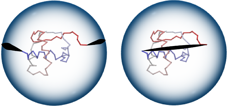
Closure using a sphere (left) and direct closure (right).
In Topoly there are five slightly different methods of closing chain using additional points on the big sphere: two deterministic and three random ones.
Deterministic closure:
closure = Closure.MASS_CENTER (closure = 1): segments are added to two endpoints in the direction “going out of center of mass”, and then connected by an arc on the big sphere;
closure = Closure.DIRECTION (closure = 5): parallel segments are added to two endpoints, and then connected by an arc on the big sphere; the direction of parallel segments is defined by user.
Random closure:
closure = Closure.TWO_POINTS (closure = 2): each endpoint is connected with a different random point on the big sphere, this is the default option;
closure = Closure.ONE_POINT (closure = 3): both endpoints are connected with the same random point on the big sphere;
closure = Closure.RAYS (closure = 4): like DIRECTION but direction is randomly chosen.
For random closure there is another parameter available: tries (default 200). It specifies how many times the operation of closing structure and checking the topology must be repeated to obtain statistics which knot type occurs the most often. Naturally it requires longer computations, but also gives more accurate information about the structure.
Structure reduction – max_cross
Next we want to simplify and reduce the structure as much as possible. This is very important because the invariant’s calculation time strongly depends on the complexity of the structure, namely on the number of crossings that it creates. The reduction is done after closing since there are known few methods for it that work well for closed chains, never changing their topology. In Topoly during reduction two methods are used.
First method is based on KMT algorithm. This algorithm removes chain elements that does not change the topology. Second method comes from classical knot theory and is based on the Reidemeister moves. The 3D structure is projected into 2D and some of the crossings found on this 2D projection, which do not affect the overall structure topology, are reduced.
Some complicated chains can still have many crossings after reduction. The calculation of their polynomial can last very long. For such situations there is the max_cross parameter (default 15). If the number of crossings after the reduction is larger than the max_cross parameter, then the calculation is stopped.
Subchain topology – structure_boundary, matrix, matrix_density, matrix_calc_cutoff and matrix_plot
If you are interested in the topology of certain parts of a chain, you can use the structure_boundary parameter. It accepts the indices of the first and the last desired aminoacids in the subchain. If you are interested in multiple such subchains, you can pass a list of such lists, i.e.:
boundaries=[[10,30],[31,50],[10,50]]
will find the topology of three subchains: indices 10-30, indices 31-50 and indices 10-50.
If you are interested in the topology of a whole spectrum of possible subchains it is even easier: just use the matrix parameter (default False). This may cause that the invariant will be calculated for all subchains of the original chain. Consequently, this can take very long to compute, therefore Topoly also contains the matrix_density (default 1) parameter which controls how precisely the space of all possible subchains will be explored. For matrix_density=1 all possible subchains are checked. For higher values passed to the matrix_density parameter, just every subchain is checked (namely subchains with a cut multiple of the matrix_density of atoms from both ends). After finding a knot with a probability higher than the matrix_calc_cutoff parameter (default 0), additional subchains with a similar length will be checked.
I.e. lets say you pass a structure with 20 atoms, matrix_density=5 and matrix_calc_cutoff=30 parameter. Then subchains 1-20, 1-15, 1-10, 1-5, 6-20, 6-15, 6-10, 11-20, 11-15 and 16-20 are checked. Imagine in 11-20 chain $3_1$ knot has been found with a probability of 35%. Then all “neigbouring” subchains a-b, where a is from 7..15 and b from 16..20, are also checked.
If you wanted much faster computation, but little risk of missing knotted subchains, we propose to use such combination of parameters: matrix_density=7 and matrix_calc_cutoff=20.
The representation of proteins’ chains in the form of a matrix leads to the discovery of slipknots (the overally unknotted structures which have a non-trivial subchain). More details in the section “Matrix”.
You can plot your matrix using the matrix_plot (default False).
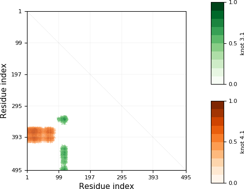
Knot matrix of exemplary structure (protein with PDB code 4M8J, chain A). Horizontal and vertical axes represent indices of respectively first and last aminoacids of particular subchain.
Calculating invariants of conjoined structures
Documentation section: Calculating invariants of conjoined structures.
In our dictionary of topological types are mainly prime structures. You may want to find polynomials of more complex structures: unjoined unions (U) and conjoined unions (#) of prime structures.
You need to create objects for your basic structures. Lets start with the 3_1 knot:
>>knot_31 = getpoly('HOMFLYPT', '3_1')
>>print(knot_31)
[+3_1: [-1 0 -2 0 [0]]|[0]|1 0 [0], -3_1: [[0] 0 -2 0 -1]|[0]|[0] 0 1]
Function finds all subtypes of the 3_1 knot and the output is the list of corresponding special objects. Each topology is represented by two values:
name (here +3_1, -3_1),
code corresponding to coefficients of its polynomial.
If you want to check what are the HOMFLYPT polynomial coefficients of +3_1 U -3_1 (unjoined union of knots) and +3_1 # -3_1 (conjoined knots) write:
>>plus_31, minus_31 = knot_31
>>plus_31 + minus_31
+3_1 U -3_1: [[0]]|-2 0 -3 [0] 3 0 2|[0]|1 0 3 [0] -3 0 -1|[0]|-1 [0] 1
>>plus_31 * minus_31
+3_1 \# -3_1: [2 0 [5] 0 2]|[0]|-1 0 [-4] 0 -1|[0]|[1]
List of such objects (e.g. polynomials=[plus_31 + minus_31, plus_31 * minus_31]) can be exported to a new dictionary file:
>>exportpoly(polynomials, exportfile='new_polvalues.py')
Gaussian Linking Number calculation (GLN)
Examples: topoly_tutorial/GLN.py.
Documentation section: GLN.
Gaussian linking number is a measure how many times one curve winds around second one, i.e. usually it can be a good measure how strongly they are linked (unfortunetely there are exceptions like Whitehead link with GLN equal to 0). If there are two closed chains, then GLN is always an integer, for instance for chains creating Hopf link:
>>gln(chain1, chain2)
-1
You can also calculate the GLN of subchains, which will be open chains - after cutting a few atoms the GLN will not be integer anymore, but close to -1:
>>gln(chain1, chain2, chain1_boundary=[5,80], chain2_boundary=[1,72])
-0.942
There are three main other options which allow more detailed calculations: maxGLN, avgGLN and matrix (all are set to False by default).
If you were interested in local entanglement between fragments of both structures you may use maxGLN argument. It will find maximal absolute GLN value between one chain1 and all fragments of chain2 and vice versa. It may also look for maximal absolute GLN value between all fragments of both chains (if parameter max_density is set to 1). But you need to be carefull while using the last option since this is very time consuming gor longer chains (time complexity O((nm)^2), where n, m chains lenghts). By default it set to -1 which causes function not to look for this global maximum. When max_density>1, then just every pair of subchains is checked (namely subchains with a cut multiple of the max_density of atoms from both ends):
>>gln(chain1, chain2, maxGLN=True)
{'whole': [0.107], 'wholeCH1_fragmentCH2': [0.872, '48-77'], 'wholeCH2_fragmentCH1':
[0.325, '11-34'], 'fragments': [], 'avg': None, 'matrix': None}
>>
>>gln(chain1, chain2, maxGLN=True, max_density=10)
{'whole': [0.107], 'wholeCH1_fragmentCH2': [0.872, '48-77'], 'wholeCH2_fragmentCH1':
[0.325, '11-34'], 'fragments': [0.901, '50-80', '10-60'], 'avg': None, 'matrix': None}
Using matrix argument you can create a matrix of GLN values between chain1 and all possible subchains of chain2 (and plot it with matrix_plot argument):
>>gln(chain1, chain2, matrix=True, matrix_plot=True)
{'whole': [0.905], 'wholeCH1_fragmentCH2': [], 'wholeCH2_fragmentCH1': [], 'fragments': [],
 'avg': None, 'matrix': #BIG TWO DIMENSIONAL MATRIX}
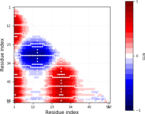
Exemplary GLN map.
Lasso type identification (minimal surface calculation)
Examples: topoly_tutorial/lasso_minimal_surface.py.
Documentation section: Lasso type indentification (minimal surface calculation).
For checking the type of a lasso topology Topoly checks how many times a lasso loop is pinned by a lasso tail. For checking if the pinning happened, Topoly calculates the minimal surface spanned on a lasso loop and checks if it is crossed. For more information look at this subpage of LassoProt database.
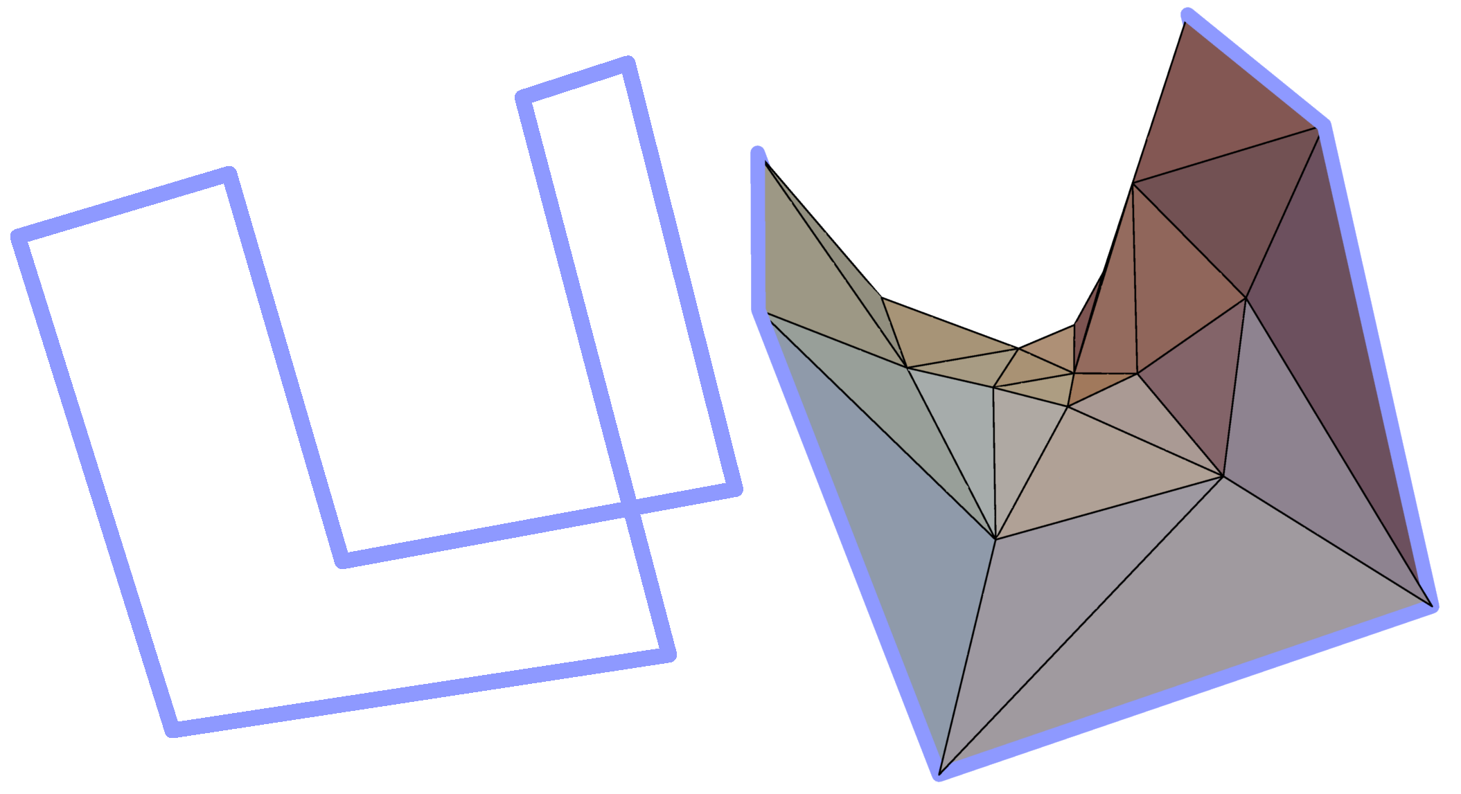
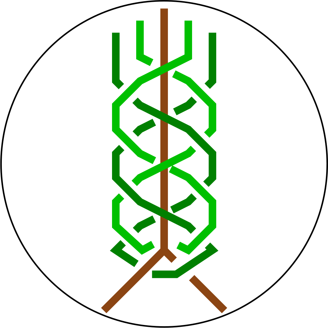
Minimal surface on an exemplary frame. Similar structures are created by soap bubbles.
For checking a lasso topology, input your structure and indices of the first and the last point of a loop.:
>>lasso_type(structure, [1,12])
{(1, 12): 'L+2C'}
Which means that through a lasso loop with indices 1-20 the tail C (last part of chain) crosses twice. Symbol ‘+’ indicates the orientation of the first crossing. For further explanation look at this subpage of LassoProt database <https://lassoprot.cent.uw.edu.pl/lasso_classification#lasso_type> _.
If your structure is in PDB format do not need to give all the loops indices, Topoly can find them:
>>lasso_type(structure)
{(1, 12): 'L+2C', (36, 60): 'L0'}
By default Topoly looks only for disulfide bridges but you can use parameter pdb_bridges to look for other covalent loops (e.g. created by amide bridges) and the bridges mediated by ions.
You can also get more information in the output (e.g. exact indices of aminoacids that cross the surface) using the parameter more_info:
>>lasso_type(structure, [1,12], more_info=True)
{(1, 12): {'class': 'L+2C', 'beforeN': [], 'beforeC': ['+25', '-27'], 'crossingsN': [], 'crossingsC': ['+25', '-27'],
'Area': 100.766, 'loop_length': 36.0001, 'Rg': 8.12732, 'smoothing_iterations': 0}}
To get the files to plot the structure with surface and crossings idicated in different tools (VMD, Jsmol, Mathematica) use parameter pic_files.
If you were only interested in a shape of minimal surface, type:
>>make_surface(structure, [1,30])
[{'A': {'x': -5.796, 'y': -0.0, 'z': 0.0}, 'B': {'x': 0.0, 'y': 0.0, 'z': 0.0}, 'C': {'x': -5.019, 'y': 2.898, 'z': 0.0}},
{'A': {'x': -5.019, 'y': 2.898, 'z': 0.0}, 'B': {'x': 0.0, 'y': 0.0, 'z': 0.0}, 'C': {'x': -2.898, 'y': 5.019, 'z': 0.0}},
{'A': {'x': -2.898, 'y': 5.019, 'z': 0.0}, 'B': {'x': 0.0, 'y': 0.0, 'z': 0.0}, 'C': {'x': -0.0, 'y': 5.796, 'z': 0.0}},
{'A':....
to get a complete information about a mesh creating a minimal surface.
Random polygons generation
Documentation section: Random polygons generation.
You can generate equilateral random walks, random loops and structures composed of them: lassos and handcuffs. Loop generation in these functions is based on Jason Cantarellas work. To generate such structures type:
>>generate_walk(30, 100)           # 100 walks of length 30
>>generate_loop(27, 100)           # 100 loops of length 27
>>generate_lasso(12, 8, 100)       # 100 lassos with loop length of 12 and tail length of 8
>>generate_handcuff([4,7], 5, 100) # 100 handcuffs with loops of length 4 and 7 and tail length of 5
>>generate_link([4,7], 2, 100)     # 100 loop pairs of length 4 and 7 and distance between their geometric centers of 2
Visualization
Documentation section: Visualization.
You can see your structure using VMD or Python’s matplotlib.
If you want to view a .xyz structure in VMD, use the function:
>>xyz2vmd('file.xyz')
it converts a .xyz file into a .pdb structure file and a .psf topology file. To open your structure in vmd, type in terminal:
>>vmd file.pdb -psf file.psf
If you want to view a structure (using matplotlib) in any of the supported formats, type:
>>plot_graph(structure)
Finding loops, theta-curves and handcuffs in structure
Examples: topoly_tutorial/import_and_find.py.
Documentation section Finding loops, theta-curves and handcuffs in structure.
If you want to find loops, theta-curves or handcuffs in your structure, type one of these functions:
>>find_loops(structure)
>>find_thetas(structure)
>>find_handcuffs(structure)
To find the corresponding topology please set the output_type parameter that selects the output type: python list, .xyz file or generator.
Matrix functions
Examples: topoly_tutorial/matrices.py.
Documentation section Knot map manipulating functions.
Matrix functions gives you more control over matrices created by gln or invariant methods.
plot_matrix prints a map after passing a matrix created by gln or one of the invariant functions (conway, homfly, etc.). It has more plotting parameters than the invariant functions giving you more control over the generated output.
find_spots(matrix) – finds geometrical centers of each identified topology field.
plot_matrix(matrix) – plots map basing on given matrix. It has more plotting parameters than invariant calculating functions, giving you more control over the generated output.
translate_matrix(matrix) – changes format of a given matrix (to dictionary or list of lists)
Data manipulation
Documentation section: Data manipulation.
There are three more functions:
find_matching translating polynomial coefficient data into topology type,
reduce_structure reducing a structure using Reidemeister moves/KMT algorithm (check Structure reduction – max_cross),
close_curve for closing an open curve (check Structure closing – closure, tries),
Examples of find_matching usage
If you have invariant a (i.e. Yamada) polynomial coefficients string use find_matching to identify the topology type:
>>find_matching('1 1 1 1 1 1 1 1 1', 'Yamada')
'2^2_1'
You can also check more complicated inputs which can be outputs of some Topoly functions – i.e. dictionary of polynomial probabilities:
>>find_matching({'1 -1 1': 0.8, '1 -3 1': 0.2}, 'Alexander')
{'3_1': 0.8, '4_1': 0.2}
or dictionary of polynomial probabilities for each subchain:
>>find_matching({(0, 100): {'1 -1 1': 0.8, '1 -3 1': 0.2}, (50, 100): {'1 -1 1': 0.3, '1': 0.7}}, 'Alexander')
{(0, 100): {'3_1': 0.8, '4_1': 0.2}, (50, 100): {'3_1': 0.3, '0_1': 0.7}}